
Convolutional neural networks (CNNs) are a fundamental architecture in data analysis, machine learning (ML). and deep learning. This guide explains how CNNs work, how they differ from other types of neural networks, their applications, and the advantages and disadvantages associated with their use.
Table of contents
- What is a CNN?
- How CNNs work
- CNNs vs. RNNs and transformers
- Applications of CNNs
- Advantages of CNNs
- Disadvantages of CNNs
What is a convolutional neural network?
A convolutional neural network (CNN) is a deep learning architecture specifically designed to process spatial data, like images and videos. CNNs use convolutional layers with filters to detect and learn hierarchical features within the input, from simple edges to complex shapes, making them highly effective for tasks such as image classification, object detection, and video analysis.
Let’s unpack this definition a bit. Spatial data is data where the parts relate to each other via their position. Images are the best example of this.
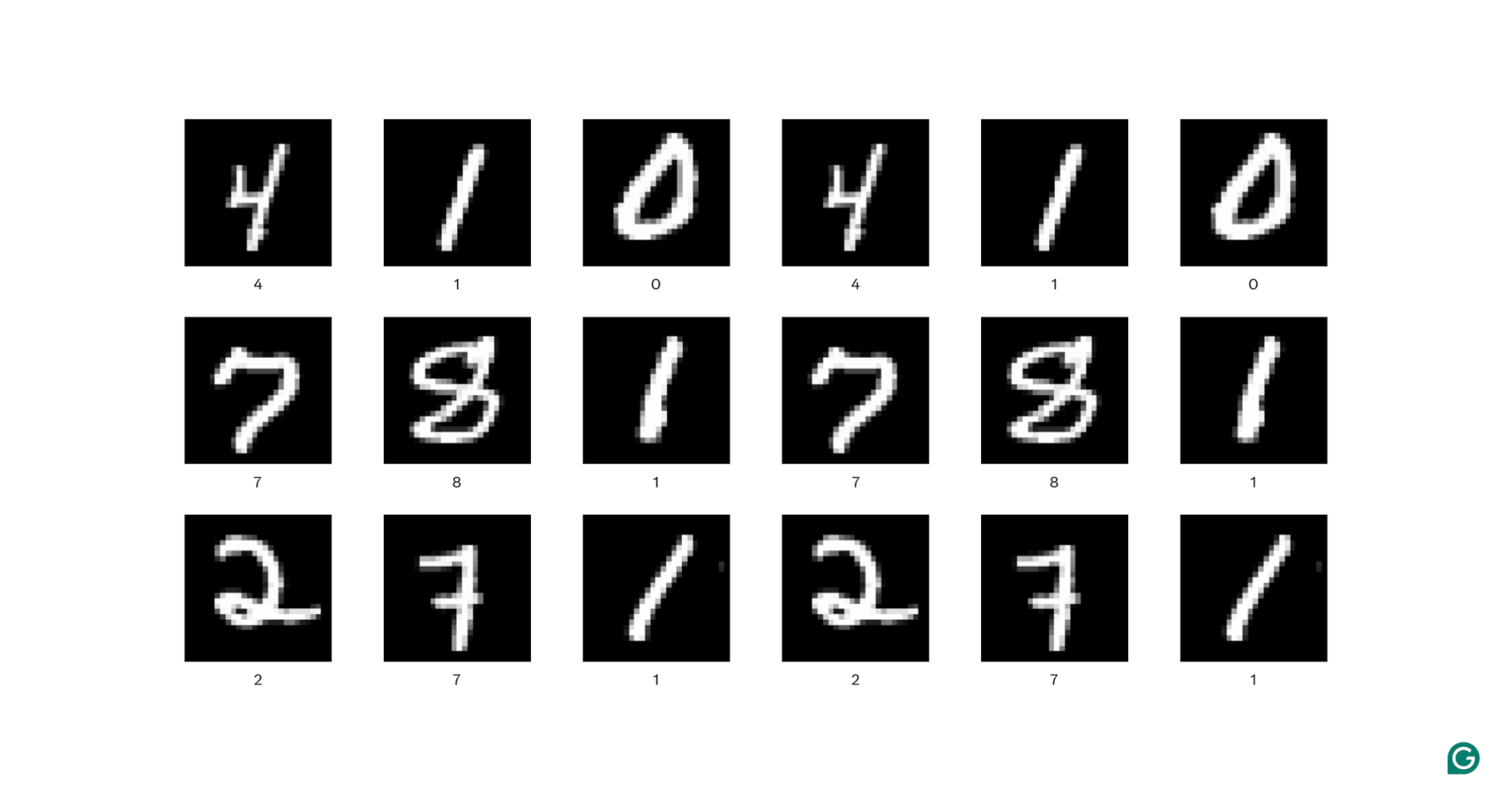
In each image above, each white pixel is connected to each surrounding white pixel: They form the digit. The pixel locations also tell a viewer where the digit is located within the image.
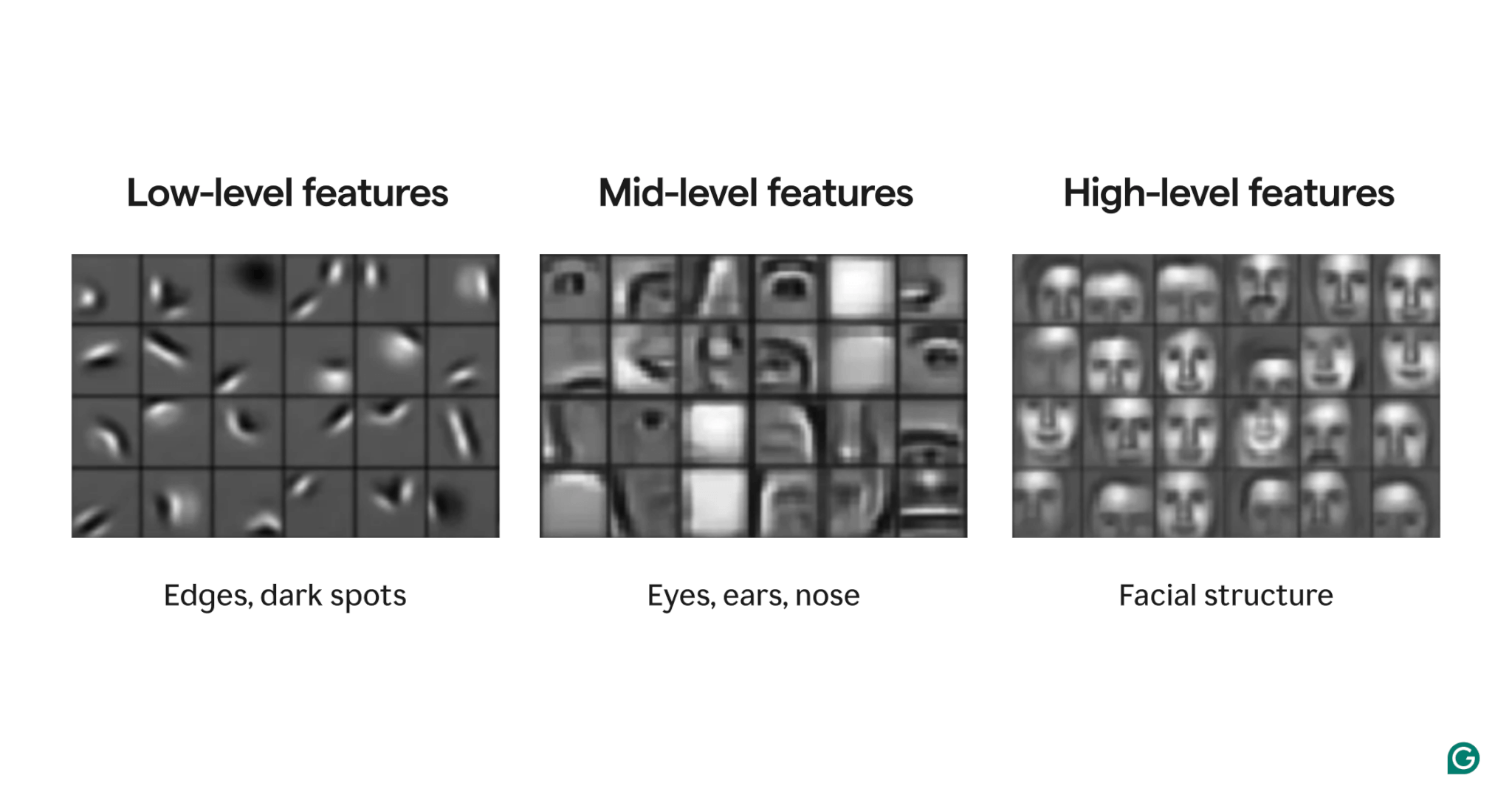
Features are attributes present within the image. These attributes can be anything from a slightly tilted edge to the presence of a nose or eye to a composition of eyes, mouths, and noses. Crucially, features can be composed of simpler features (e.g., an eye is composed of a few curved edges and a central dark spot).
Filters are the part of the model that detects these features within the image. Each filter looks for one specific feature (e.g., an edge curving from left to right) throughout the entire image.
Finally, the “convolutional” in convolutional neural network refers to how a filter is applied to an image. We’ll explain that in the next section.
CNNs have shown strong performance on various image tasks, such as object detection and image segmentation. A CNN model (AlexNet) played a significant role in the rise of deep learning in 2012.
How CNNs work
Let’s explore the overall architecture of a CNN by using the example of determining which number (0–9) is in an image.
Before feeding the image into the model, the image must be turned into a numerical representation (or encoding). For black-and-white images, each pixel is assigned a number: 255 if it’s completely white and 0 if it’s completely black (sometimes normalized to 1 and 0). For color images, each pixel is assigned three numbers: one for how much red, green, and blue it contains, known as its RGB value. So an image of 256×256 pixels (with 65,536 pixels) would have 65,536 values in its black-and-white encoding and 196,608 values in its color encoding.
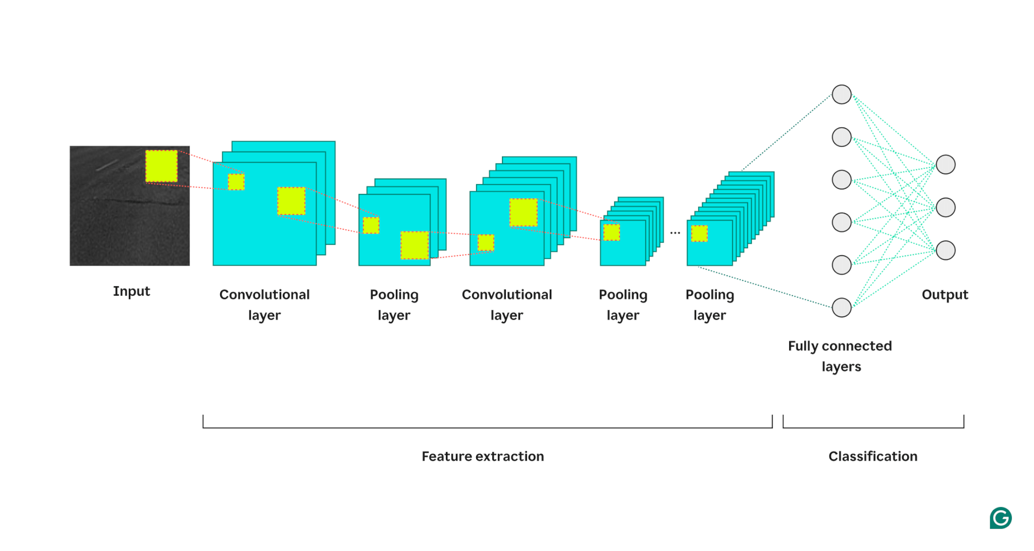
The model then processes the image through three types of layers:
1 Convolutional layer: This layer applies filters to its input. Each filter is a grid of numbers of a defined size (e.g., 3×3). This grid is overlaid on the image starting from the top left; the pixel values from rows 1–3 in columns 1–3 will be used. These pixel values are multiplied by the values in the filter and then summed. This sum is then placed in the filter output grid in row 1, column 1. Then the filter slides one pixel to the right and repeats the process until it has covered all rows and columns in the image. By sliding one pixel at a time, the filter can find features anywhere in the image, a property known as translational invariance. Each filter creates its own output grid, which is then sent to the next layer.
2 Pooling layer: This layer summarizes the feature information from the convolution layer. The convolutional layer returns an output larger than its input (each filter returns a feature map approximately the same size as the input, and there are multiple filters). The pooling layer takes each feature map and applies yet another grid to it. This grid takes either the average or the max of the values in it and outputs that. However, this grid doesn’t move one pixel at a time; it will skip to the next patch of pixels. For example, a 3×3 pooling grid will first work on the pixels in rows 1–3 and columns 1–3. Then, it will stay in the same row but move to columns 4–6. After covering all the columns in the first set of rows (1–3), it will move down to rows 4–6 and tackle those columns. This effectively reduces the number of rows and columns in the output. The pooling layer helps reduce complexity, makes the model more robust to noise and small changes, and helps the model focus on the most significant features.
3 Fully connected layer: After multiple rounds of convolutional and pooling layers, the final feature maps are passed to a fully connected neural network layer, which returns the output we care about (e.g., the probability that the image is a particular number). The feature maps must be flattened (each row of a feature map is concatenated into one long row) and then combined (each long feature map row is concatenated into a mega row).
Here is a visual representation of the CNN architecture, illustrating how each layer processes the input image and contributes to the final output:
A few additional notes on the process:
- Each successive convolutional layer finds higher-level features. The first convolutional layer detects edges, spots, or simple patterns. The next convolutional layer takes the pooled output of the first convolutional layer as its input, enabling it to detect compositions of lower-lever features that form higher-level features, such as a nose or eye.
- The model requires training. During training, an image is passed through all the layers (with random weights at first), and the output is generated. The difference between the output and the actual answer is used to adjust the weights slightly, making the model more likely to answer correctly in the future. This is done by gradient descent, where the training algorithm calculates how much each model weight contributes to the final answer (using partial derivatives) and moves it slightly in the direction of the correct answer. The pooling layer does not have any weights, so it’s unaffected by the training process.
- CNNs can work only on images of the same size as the ones they were trained on. If a model was trained on images with 256×256 pixels, then any image larger will need to be downsampled, and any smaller image will need to be upsampled.
CNNs vs. RNNs and transformers
Convolutional neural networks are often mentioned alongside recurrent neural networks (RNNs) and transformers. So how do they differ?
CNNs vs. RNNs
RNNs and CNNs operate in different domains. RNNs are best suited for sequential data, such as text, while CNNs excel with spatial data, such as images. RNNs have a memory module that keeps track of previously seen parts of an input to contextualize the next part. In contrast, CNNs contextualize parts of the input by looking at its immediate neighbors. Because CNNs lack a memory module, they are not well-suited for text tasks: They would forget the first word in a sentence by the time they reach the last word.
CNNs vs. transformers
Transformers are also heavily used for sequential tasks. They can use any part of the input to contextualize new input, making them popular for natural language processing (NLP) tasks. However, transformers have also been applied to images recently, in the form of vision transformers. These models take in an image, break it into patches, run attention (the core mechanism in transformer architectures) over the patches, and then classify the image. Vision transformers can outperform CNNs on large datasets, but they lack the translational invariance inherent to CNNs. Translational invariance in CNNs allows the model to recognize objects regardless of their position in the image, making CNNs highly effective for tasks where the spatial relationship of features is important.
Applications of CNNs
CNNs are often used with images due to their translational invariance and spatial features. But, with clever processing, CNNs can work on other domains (often by converting them to images first).
Image classification
Image classification is the primary use of CNNs. Well-trained, large CNNs can recognize millions of different objects and can work on almost any image they’re given. Despite the rise of transformers, the computational efficiency of CNNs makes them a viable option.
Speech recognition
Recorded audio can be turned into spatial data via spectrograms, which are visual representations of audio. A CNN can take a spectrogram as input and learn to map different waveforms to different words. Similarly, a CNN can recognize music beats and samples.
Image segmentation
Image segmentation involves identifying and drawing boundaries around different objects in an image. CNNs are popular for this task due to their strong performance in recognizing various objects. Once an image is segmented, we can better understand its content. For example, another deep learning model could analyze the segments and describe this scene: “Two people are walking in a park. There is a lamppost to their right and a car in front of them.” In the medical field, image segmentation can differentiate tumors from normal cells in scans. For autonomous vehicles, it can identify lane markings, road signs, and other vehicles.
Advantages of CNNs
CNNs are widely used in the industry for several reasons.
Strong image performance
With the abundance of image data available, models that perform well on various types of images are needed. CNNs are well-suited for this purpose. Their translational invariance and ability to create larger features from smaller ones allow them to detect features throughout an image. Different architectures are not required for different types of images, as a basic CNN can be applied to all kinds of image data.
No manual feature engineering
Before CNNs, the best-performing image models required significant manual effort. Domain experts had to create modules to detect specific types of features (e.g., filters for edges), a time-consuming process that lacked flexibility for diverse images. Each set of images needed its own feature set. In contrast, the first famous CNN (AlexNet) could categorize 20,000 types of images automatically, reducing the need for manual feature engineering.
Disadvantages of CNNs
Of course, there are tradeoffs to using CNNs.
Many hyperparameters
Training a CNN involves selecting many hyperparameters. Like any neural network, there are hyperparameters such as the number of layers, batch size, and learning rate. Additionally, each filter requires its own set of hyperparameters: filter size (e.g., 3×3, 5×5) and stride (the number of pixels to move after each step). Hyperparameters cannot be easily tuned during the training process. Instead, you need to train multiple models with different hyperparameter sets (e.g., set A and set B) and compare their performance to determine the best choices.
Sensitivity to input size
Each CNN is trained to accept an image of a certain size (e.g., 256×256 pixels). Many images you want to process might not match this size. To address this, you can upscale or downscale your images. However, this resizing can result in the loss of valuable information and may degrade the model’s performance.


