Arik Motskin, Michael Haugan, and Parth Aidasani from Grammarly’s Data Science team co-wrote this article.

Strategic investment in paid advertising has fueled Grammarly’s user base growth to over 30 million daily active users. However, as our rapid growth continues, it’s crucial that the Acquisition Marketing and Data Science teams rigorously evaluate the impact and efficiency of our ad spend across channels.

To pressure-test our assumptions, we built a geo-experimentation framework to measure the incrementality of various ad channels, focusing initially on YouTube marketing. This approach blends our internal knowledge and domain expertise with today’s industry-leading concepts and technical approaches. We’re excited to dive into how we developed the framework, important considerations, and its direct applications to our business.

The Challenge of Attribution

Geo experimentation, where users are exposed to different experimental conditions based on their geographic location, has been used for several years in the industry (as an example, consider [study results reported in 2016]), proving its value as a way to measure the incrementality of marketing channels. But given the relative complexity and high setup costs, why are geo experiments necessary? It all comes down to the challenge of attribution, which is the problem of assigning credit to marketing channels for every newly acquired user.

Traditional attribution primarily focuses on first-touch, last-touch, or Multi-Touch Attribution and can be effective for down-funnel or click-based channels such as search. However, top-of-funnel channels that drive views instead of clicks, such as digital video and TV, tend to be under-credited. Geo experiments do not rely on digital touchpoints, allowing us to measure the impact of top-of-funnel media and brand ads, which most marketers struggle with. Moreover, these experiments help us measure the impact channels drive throughout the funnel and on other channels, known as the “halo effect,” which is often ignored with traditional attribution models.

Even if we were to consider every touchpoint along the user journey, we could still fail to measure the net incremental impact driven by a channel. While it is fair to assume that users frequently convert because they saw an ad, this is only sometimes the case, especially with larger companies with good brand equity. For example, if a user first sees several YouTube ads but later goes to a search engine, searches for Grammarly, and converts from there, the search channel would get credit on paper even though we know that search did not cause the conversion. A geo experiment would help us uncover whether YouTube played a role in having the user convert or whether the user would have converted anyway without ever seeing those YouTube ads.

Finally, with the deprecation of third-party cookies looming, measurement and attribution become increasingly challenging due to the lack of comprehensive tracking, especially across upper-funnel media. Marketers must increasingly rely on these tests to uncover a channel’s incremental effects.

High-Level Methodology

The basic idea of geo experimentation is quite simple: divide users into a set of geographic “units” that cover a target market, like the set of Designated Market Areas (DMAs) in the US. For some carefully specified testing period, a portion of these geographic units (the “control” set) continue receiving the current level of channel marketing spend. In contrast, another portion of the units (the “test” set) has its channel marketing spend “go dark” or turned off completely. At the conclusion of the testing period, we measure KPIs for each set and determine whether marketing spend provides a statistically significant lift and, if so, by how much.

Sounds straightforward enough, but the devil is truly in the details. For instance, not just any control and test sets will do. Ideally, we can identify a good “split” or two sets of geographic units so similar across our KPIs and other dimensions that any performance difference throughout the experiment can be attributed to the change in marketing spend. When deciding on the size of these sets, one needs to balance the benefit of additional statistical power with the opportunity cost and business disruption that a large “go-dark” experiment can cause.

Related to the size of the sets is the length of the experiment. A longer experiment generates more data, can provide a more accurate estimate of incremental lift, and may even reveal seasonal patterns in the incremental lift itself. With top-of-funnel channels like video, where a user may require repeated marketing exposures to convert, a longer experiment window can better account for this lag.

But with a longer experiment comes the challenge of business disruption and the very real risk of drift in your split, where the control and test geographic units become less similar over time due to factors like demographic/economic shifts or major one-off local events. This needs to be monitored and accounted for as well.

KPIs

Traditionally, the most common KPIs in consumer acquisition are sign-ups, new active users, revenue, or LTV. While having a monetary KPI like revenue is ideal for enabling better ROI measurement and decision-making, revenue is not the best KPI for Grammarly in this instance. This is because Grammarly employs a freemium model, where users often sign up for the free tier before upgrading to the Premium paid tier.

Media spend is typically not a direct driver of Premium purchases due to the lag between the sign-up and the upgrade. As a result, we chose new active users as the primary metric, as it is not too deep in the funnel and is still very relevant to the business. This makes measurement during our test period far more feasible, as the typical window between an ad impression and a new active user is within our test period.

Measurement Strategy

To conduct measurement for this experiment, we leverage causal inference to build a counterfactual that predicts the performance of our KPI—new active users—as if YouTube media never went dark and continued business as usual. This counterfactual will be compared to what actually happens to understand the channel’s incremental impact.

For this experiment, we deployed Google’s open-source TBR package for time-series model building due to its focus on experimentation, although we first considered the CausalImpact package, which is better suited for causal inference with observational data. The approach works as follows: given a control and test population and a time series of pre-intervention historical data for a given metric for both control and test groups, we compute a synthetic baseline for the post-intervention period based on a Bayesian structural time series (BSTS) model. The baseline includes point estimates (i.e., the predicted “counterfactual”) and daily confidence intervals. By building this synthetic baseline in the post-intervention period, we can later compare the actual test performance against the synthetic baseline to determine the KPI lift.

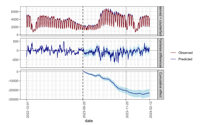
This chart shows the daily and aggregate difference between observed values in a test set and the predicted (synthetic baseline) values in that test set. The synthetic baseline is constructed via a BSTS model trained on historical data in our splits.

Geo Split Selection

When building our split, our preferred geographic unit is the Designated Market Area (DMA). The 210 DMAs that cover the United States—originally defined by Nielsen for television and radio markets—represent distinct, mostly self-contained markets. A key property of the DMA model is that a typical user will not cross the boundary of their DMA over the course of a day, unlike with states or metropolitan areas. This property is critical to the success of a geo experiment. Otherwise, there is an increased risk that individuals may be in different experiment regions at different times of day, which introduces noise. For example, an individual could be at home in the morning in a go-dark region but view advertisements in another region during the day while at work.

But with 210 DMAs, there are roughly 10⁶² ways to split this set into two groups of 105 DMAs each (not to mention countless ways to split into an uneven number per group), so we definitely need to prune the tree of possibilities to make split selection tractable. As such, we employed two separate methods for split generation:

i) Clustering: To generate candidate splits that are likely to be somewhat balanced, we first sort DMAs into buckets based on their average historical KPI values. Within each bucket, we randomly sample two DMAs (one for test, one for control) until all DMAs have been assigned. This approach ensures that we have a reasonably good starting point when evaluating candidate splits.

ii) Randomization: Unlike clustering, a randomized method does not pre-classify DMAs and instead selects DMA splits randomly, regardless of size. This approach addresses the concern that clustering may result in local maxima, as randomizing allows us to explore other parts of the search space. After all, a split can be balanced overall, even if it is not pairwise balanced at the DMA level.

Geo Split Evaluation

Now that we have generated a large set of candidate splits from each of the above methods, we must choose a balanced split among all the candidates to use in the experiment. For each candidate, we used two metrics to evaluate its quality. Firstly, we considered the historical similarity in a split; in particular, we computed our KPI’s historical RMSE (root-mean-square error) between split pairs after normalizing for total KPI volume. This offers a backward-looking comparison, which is important but certainly not sufficient.

Secondly, we looked at the predicted performance of the Bayesian time-series structural model for each split. That is, we measured how closely the KPI of a predicted synthetic baseline of the test DMAs (i.e., the counterfactual) compares to the real KPI of the test DMAs, measured in a historical training and test period. Ideally, we picked a split where the time-series model can accurately predict the (non-intervention) performance of the KPI metric. An added benefit of this approach is that it allows us to compute the potential drift in a selected split; that is, while two sets of DMAs may initially be quite similar, they may begin to diverge gradually over time. Fortunately, we found that drift was mostly minimal in the highest-performing splits over a three to six-month test window. Based on these criteria, we picked the highest-performing split to use in our go-dark experiment, which was a split generated by the Randomization method above. As a result, DMAs in the control and test sets were not pairwise balanced as with candidates from the Clustering method. However, the sets were extremely balanced in aggregate, both historically and in predicted performance.

Power Analysis

When determining the sensitivity of a geo experiment, we have two levers at our disposal: the size of the control and test sets (i.e., the percent of all DMAs diverted to the experiment) and the length of the experiment. Our goal was to determine how to select these parameters for an accurate lift measurement.

For a fixed set size and experiment length (e.g., 50% of all DMAs, with the experiment running for 12 weeks), we determined the sensitivity of the experiment as follows:

1 After identifying the top-performing split according to the methodology above, we use TBR to generate a synthetic baseline for the test KPI metric post-intervention date. On day i, we call the synthetic KPI value SyntheticTest_i and the true realized historical value RealizedTest_i.

2 For a lift value k% drawn from a spectrum of possible lift values (1%, 2%, 3%, etc.}, simulate a lift of this size by setting SimulatedTest_i = RealizedTest_i * (100-k%) ± N(0,σ²). The normally distributed noise term is fit according to a historical estimate of the KPI variance.

3 Finally, we check whether this simulated set of KPI values would be detected as a statistically significant lift (or drop) above (or below) the SyntheticTest values, repeating this simulation 1,000 times across all desired DMA and test length parameters.

Besides sensitivity, it was also critical to estimate the opportunity cost of each parameter choice; after all, while a long experiment may help gather insightful data points, there are business consequences to going dark for an extended period. We estimated the potential opportunity cost of each parameter selection as a function of the derived lift sensitivity values, the average KPI values in the experiment DMAs, and the test length.

Results and Applications

Our experiment yielded many new insights that could change how we treat ads throughout the year. Before Grammarly’s typical seasonal peak, we found a substantial incremental lift in our KPI between the control and go-dark groups. However, the incremental lift noticeably moderates during the seasonal peak before rising again afterward.

Furthermore, we can improve our understanding of our media efficiency by considering incremental cost per new user instead of just cost per new user. This provides better insight into our most efficient channels and where to invest our next media dollars. To compute these incremental cost metrics, we built a counterfactual spend for our test set via the TBR model as if we had never turned off spend in this channel.

This proved to be a fortuitous decision. Like many companies, Grammarly usually ramps up spend during these seasonal peaks, and we found that our efficiency significantly worsened during these seasonal moments due to increased spend levels and lower incremental KPI lift. Our hypothesis is that there are organic, non-marketing forces that compel users to join Grammarly during these high seasonal moments, so our ads are not driving as much incremental impact during these periods.

Interestingly, we did not observe any meaningful signs of lag in our test, as a KPI lift was evident shortly after the intervention went live. One intriguing hypothesis is that this video channel is potentially more down-funnel-heavy than we had previously assumed. On the other hand, due to the volatile seasonal changes in our KPI metric that we discovered, our test may have lacked the sensitivity to isolate the lag effect that creeps in over time.

Closing Thoughts

Our geo-based, go-dark experimental approach gave us deep, new insights into the actual incremental impact of media channels. In particular, we now better understand the ROI, seasonality, and lag in Grammarly’s marketing efforts. It helps acquisition leaders better address the question “Where should my next dollar go?” and provides a robust tool for impact measurement in our increasingly cookie-less world. If you are excited by the prospect of leveraging cutting-edge data science to tackle challenges like marketing effectiveness, check out our open positions and become a part of our trailblazing journey.